Final Report
Contextual Robust Word Recognition
Zhao Cheng, Benjamin Walker
Summary
Our project is a robust word recognition system specifically for low quality images. This report discusses the results and methods of character and word recognition to achieve the project objectives.
Results Overview
Successful implementation of contextual based word recognition with 28.84% error rate. Four classification methods were written by the team for character recognition. These are Artificial Neural Network (ANN), Decision Tree, k Nearest Neighbor (kNN), Support Vector Machine (SVM). The following table contains the classification error rate and run time for each method.
|
Algorithm |
Error Rate(%) |
Run Time (sec) |
|
SVM |
33.97 |
135 |
|
D-Tree |
20.41 |
60 |
|
kNN |
10.05 |
30 |
|
ANN (Toolbox) |
19.67 |
1200 |
|
ANN (self-written) |
10.85 |
54 |
Methodology
Character recognition is achieved through the completion of four tasks. These tasks are image processing, word segmentation, feature extraction, classifier design and training. The classifier with the lowest error rate was chosen to supply labeled characters to the Word Recognition algorithm.
Image processing
The objective of image processing is to read the image data files and output the segmented character images. Four steps are needed in this process, and the first step is to read data into image matrices from image file folder. Then, an unsurprised clustering algorithm is used to separate the word from its background. The word image is then transformed from a color image into a black-white image. In order to segment the words into individual characters, a region connection algorithm is implemented. In the last step, the word is cut into several characters image. Some other methods such as checking area of connected region are also applied to make this process more robust to the noise. Here is an example,
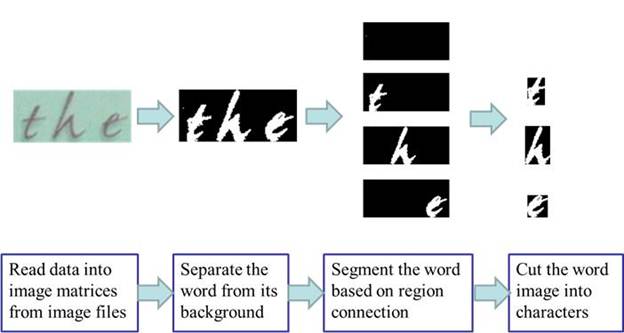
Figure 1: Image processing procedure
Feature Extraction
There are many methods available to extract the feature of a character image. Among all these existing methods, taking pixels directly out is perhaps the simplest and most straight forward one. However, it is not possible to take pixels directly as size of character images varies for different samples. In order to address this problem, we will take the pixels from a resized 10 by 10 image,. Note that it is not necessary to set the normalized size to be 10 by 10, as the Matlab function GenerateDataset is designed to deal with any output size. From the figure, it is easy to show that by downsizing the image, some of the critical information is lost. However, the size cannot be too large as the amount of sample data grows squarely to the size, increasing computation time.
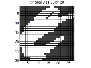
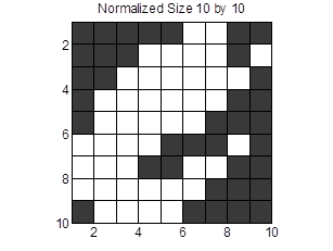
Figure 2: Example of a character image, left original image, right normalized image
Shape context
Shape context is a method that allows for measuring shape similarity between two images. We can extract two scores as the measurements of similarity, the affine score and the shape-context score. This can be treated as the distance of two samples which allows predictions with the k-nearest neighbor method. We downloaded the source code from the original inventor and implement it in character recognition [5].
Figure 3: One hundred sample features are extracted per example. Each dot corresponds to a feature. Shape context is based on comparison of features.
Classifier Design
Four classification algorithms have been written and implemented with varying degrees of success.
Support Vector Machine (SVM)
The SVM is based on problem 1 homework 3, but modified to implement 26 binary classifiers. These classifiers pass an individual prediction to a decision fusion function. There are three possible outcomes from the classifiers:
· One classifier returns a label
· None of the classifiers return a label
· More than one classifier returns a label.
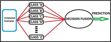
Figure 4: Design scheme for Multiclass SMV
The decision fusion currently handles the first two outcomes. If a single classifier returns a positive label, then the prediction is that label. If none of the classifiers return a positive label, there is no prediction, and the example is recorded as a classification error. There is not an error handling case for the 3rd case. This case is future work. The error rate for each individual classifier (a-z) is below.
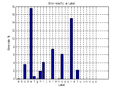
Figure 5: SVM individual binary classifier error rate. This is the error rate of an individual classifier (A-Z) predicting one character over the entire dataset.
Decision Tree
Decision Tree is based on the binary
classifiers from the homework. However, this code does not work properly unless
we modify it so that it is capable to make predictions for multiple classes.
The modification includes two functions, the function impurity in which
we calculate the impurity and the function declare_leaves in which
multi-class comparison is considered. We have also tested the performance
with 5-folder cross validation method on the training dataset. In order to
acess the parameters for this method, we have designed the following possible
values for parameter ![]() . The figure below
graphs the error rate for increasing values of the C parameter.
. The figure below
graphs the error rate for increasing values of the C parameter.
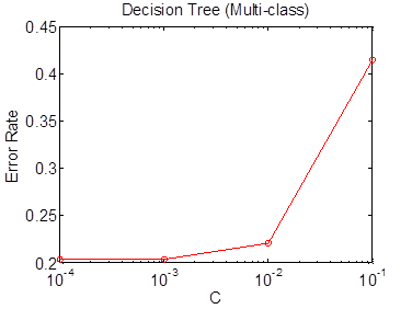
Figure 6: D-Tree error rate versus (C) parameter. These results are used to determine the optimal (C) parameter at 1e-3.
k Nearest Neighbor (kNN)
The kNN is based on problem 4 of homework 1, but is modified to handle multiple classes. A k value of 5 was determined optimal experimentally. The kNN is implemented using a 10 cross-fold validation. Multiple class positive returns are handled by a recursive call with a decreasing k value. This error handling scheme overlooks the cases where two labels with similar features, for example, (i) and (l), have an imbalance in the number of examples. For example, (i) has 40 examples in a dataset, but (l) has 200. So when the features of a test sample are compared, the number of (l) may swamp out the correct reading of (i) when it comes to tallying the votes. A possible solution would be to examine the top 2 most frequent labels, and perform a recursive ‘error’ check, and comparing the (k=1) vote to the current k value prediction, weighting each k value vote based upon the feature distance.
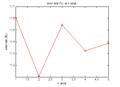
Figure 7: kNN error rate versus k-value. Optimum k-value of 5 determined experimentally.
Artificial Neural Network (ANN)
Artificial neural network is also implemented. The neural network we developed has 100 input nodes as each sample data has 100 attributes. A hidden layer is assigned with 50 nodes. Only one node is assigned as the output. This design will enforce all 26 difference classes share one output node. In order to distinguished between multiple classes, the output nodes uses index number 1 to 26. This may induce output confusing as the relation in adjacent indexed classes does not exist. The error is as high as around 0.6 due to this fact.
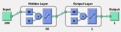
Figure 8: ANN design scheme, type 1.
An alternative design scheme in order to get rid of this output confusing problem is to assign 26 output nodes. At the same time, we also find that the neural network generated from the Matlab function newff has difficulty in handling large amount of data. A different function named feedforwardnet is called instead. With proper configuration, I setup the feed forward neural network with gradient descent with momentum back propagation. It has a satisfying performance with 19.67% error rate. The execution time is about 20 minutes with 5000 epochs.
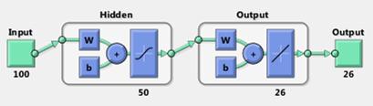
Figure 9: ANN design scheme, type 2.
After the poster presentation, we write the feed forward neural network with gradient descent with momentum back propagation by ourselves. It beats the same algorithm provided in Matlab Toolbox in both performance and execution time. It reaches 80% training accuracy within 10 epochs. The execution time for self-written program is much less than the Matlab toolbox function feedforwardnet. We find that this algorithm might cause over-fitting if the training accuracy is too high. In order to identify the best parameter, we induce performance evaluation along different parameters. The figure below shows that the parameter (acc=97.5) yields the best performance.
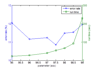
Figure 10: ANN error rate (blue) versus parameter and run time (green) versus parameter. Under-fitting occurs at parameter less than 95.5, and over-fitting occurs at parameter greater than 98.5.
Contextual based Word Recognition
With all the character recognized from the methods introduced in the previous section, we can do the word recognition by combining these character recognition results. The error rate of classification at words is higher than that at characters, because a word is regarded as error classification if any character in the word is not recognized correctly. In order to minimize the error, we apply the contextual based word recognition by comparing our classification result with a real dictionary. Every word in the dictionary is compared with the test sample word. The final prediction is determined by maximizing the likelihood. The formula below is used to calculate the maximum likelihood.
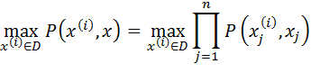
In this equation P(α,β) is the
transitional probability of character α being classified as β.
Generally, this transitional probability is not reversible P(α,β)=P(β α).
This transitional probability of each letter shows the habit of
misclassification for a classifier. The graph below illustrates the probability
for each character to be misclassified for another. This information is
used in the word prediction step to choose the most likely word.
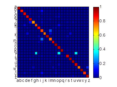
Figure 11: The x and y axes are the alphabet, and the color scale from red (high probability) to dark blue (low probability) is the transitional probability that one character is classified as another.
Result
Character Recognition
In order of assess the performance of each classifier. We run these classifiers on the dataset with 5-fold cross validation. The figure and table below shows the error rate and run time for each method.
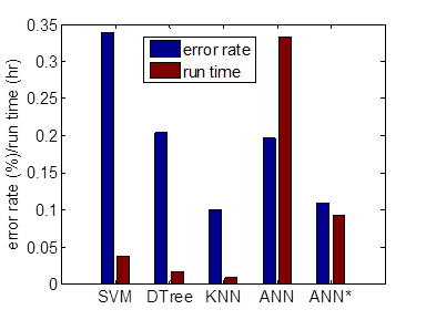
Figure 12: Error rate of individual classifier algorithm and run time. (ANN* is team written algorithm)
From the performance comparison, we find that KNN is the best algorithm to do character classification by beating others with the lowest error rate (10.05%) and the shortest run time (30sec), it is followed with the ANN (feed forward network with back propagation). Note that the error rate at words is higher than that at characters. So in this case, the word classification error rate based on KNN rises to 41.40%. In the word recognition section, we will show how much this error rate is decreased with the help of context.
Table 1 Performance of character recognition
|
Algorithm |
Error Rate(%) |
Run Time (sec) |
|
SVM |
33.97 |
135 |
|
D-Tree |
20.41 |
60 |
|
kNN |
10.05 |
30 |
|
ANN (Toolbox) |
19.67 |
1200 |
|
ANN (self-written) |
10.85 |
54 |
Word Recognition
We have 615 word images in our dataset. We take the first 400 words as the training set and the rest 215 words as the testing set. The table below shows how maximum likelihood algorithm worked for correcting the misclassified word. In order to handle the misclassification situation that is not appeared in the training set, we add the smoothing factor of 10^-5 to the transitional probability.
Table 2 Contextual based Word Recognition with likelihood determining the word prediction.
|
|
|
|
|
|
|
orance |
likelihood |
|
iast |
likelihood |
|
orange orange trance |
0.0470 0.0470 0.0029 |
|
last last east |
0.2026 0.2026 0.0111 |
|
|
|
|
|
|
|
digltal |
likelihood |
|
uniyersity |
likelihood |
|
digital |
0.0671 |
|
university |
0.0617 |
Word choice is determined by comparing the recombined characters with the dictionary. In cases of errors, the maximum likelihood of character mislabeling is used to determine the predicted word. The table below shows the error rate for each process of word recognition. At the end of the character recognition process, the error rate is very high. We then apply maximum likelihood with smoothing to reduce errors to 28.84%.
Table 3 Error rate of word recognition
|
Method |
Error Rate(%) |
|
Character Recognition |
41.40 |
|
Maximum Likelihood |
33.02 |
|
M.L. w/ smoothing |
28.84 |
Future Directions
Here we list several directions we can work on for robust word recognition problem.
· Improve error handling with the SVM in the case that no binary classifier returns a label.
· Create a general method to handle word comparison, e.g. take into account the character recognition confidence.
· Implement Hidden Markov Method with word recognition to see if it increases accuracy.
· Perform test runs with higher resolution bitmap images to determine optimum balance between resolution and run time.
Coding
The code was written entirely in Matlab. By section:
· Dataset Generation
o Word image data files from [1]
o GenerateDataset.m: team written
o parseXML.m: code from mathworks website
· Image Processing:
o ImPreProcess.m :team written
o ImLabel.m:team written
· Shape Context
o Algorithm and code from web: [5]
· Classifiers
o ANN*: team written
o ANN: calls matlab toolbox function
o D-Tree: team written, based on homework template code
o kNN: team written
o SVM: team written
· Word Recognition
o test_word.m: Team written
o test_prep.m: Team written
o 3esl.txt: dictionary word list from [8]
References
[1] ICDAR 2003 Competitions website, http://algoval.essex.ac.uk/icdar/
[2]
ICDAR 2005 Competitions website, http://algoval.essex.ac.uk:8080/icdar2005/
[3] ICDAR 2011 Competitions website, http://www.cvc.uab.es/icdar2011competition/
[4] A Shahab, F Shafait, A Dengel, "ICDAR 2011 Robust Reading Competition Challenge 2: Reading Text in Scene Images," International Conference on Document Analysis and Recognition (ICDAR), 2011 , pp.1491-1496, 18-21 Sept. 2011
[5] S Belongie, J Malik, J Puzicha, "Pattern Analysis and Machine Intelligence", IEEE Transactions on Pattern Analysis and Machine Intelligence, 24 (4), 509-522
[6] Yuxi Zhang, "Optical Word Recognition", CS 74/174 - Spring 2012, final report of term project
http://www.cs.dartmouth.edu/~lorenzo/teaching/cs174/Archive/Spring2012/Projects/Final/yuxi_zhang/final_yuxi.html
[7] Jonathan Connell and Vijay Kothari, "Handwritten Character Recognition", CS 74/174 - Spring 2012, final report of term project
[8] dicts word lists http://wordlist.sourceforge.net/12dicts-readme-r5.html